Motion – Study Material

In everyday life, we see some objects at rest and others in motion. Birds fly, fish swim, blood flows through veins and arteries and cars move. Atoms, molecules, planets, stars and galaxies are all in motion. We often perceive an object to be in motion when its position changes with time. However, there are situations where the motion is inferred through indirect evidences. For example, we infer the motion of air by observing the movement of dust and the movement of leaves and branches of trees. What causes the phenomena of sunrise, sunset and changing of seasons? Is it due to the motion of the earth? If it is true, why donít we directly perceive the motion of the earth? An object may appear to be moving for one person and stationary for some other. For the passengers in a moving bus, the roadside trees appear to be moving backwards. A person standing on the roadñside perceives the bus alongwith the passengers as moving. However, a passenger inside the bus sees his fellow passengers to be at rest. What do these observations indicate? Most motions are complex. Some objects may move in a straight line, others may take a circular path. Some may rotate and a few others may vibrate. There may be situations involving a combination of these. In this chapter, we shall first learn to describe the motion of objects along a straight line. We shall also learn to express such motions through simple equations and graphs. Later, we shall discuss ways of describing circular motion.

8.1 Describing Motion

We describe the location of an object by specifying a reference point. Let us understand this by an example. Let us assume that a school in a village is 2 km north of the railway station. We have specified the position of the school with respect to the railway station. In this example, the railway station is the reference point. We could have also chosen other reference points according to our convenience. Therefore, to describe the position of an object we need to specify a reference point called the origin.

8.1.1 MOTION ALONG A STRAIGHT LINE

The simplest type of motion is the motion along a straight line. We shall first learn to describe this by an example. Consider the motion of an object moving along a straight path. The object starts its journey from O which is treated as its reference point (Fig. 8.1). Let A, B and C represent the position of the object at different instants. At first, the object moves through C and B and reaches A. Then it moves back along the same path and reaches C through B.

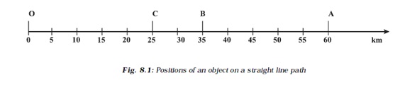
The total path length covered by the object is OA + AC, that is 60 km + 35 km = 95 km. This is the distance covered by the object. To describe distance we need to specify only the numerical value and not the direction of motion. There are certain quantities which are described by specifying only their numerical values. The numerical value of a physical quantity is its magnitude. From this example, can you find out the distance of the final position C of the object from the initial position O? This difference will give you the numerical value of the displacement of the object from O to C through A. The shortest distance measured from the initial to the final position of an object is known as the displacement Can the magnitude of the displacement be equal to the distance travelled by an object? Consider the example given in (Fig. 8.1). For motion of the object from O to A, the distance covered is 60 km and the magnitude of displacement is also 60 km. During its motion from O to A and back to B, the distance covered = while the magnitude of displacement = 35 km. Thus, the magnitude of displacement (35 km) is not equal to the path length (85 km). Further, we will notice that the magnitude of the displacement for a course of motion may be zero but the corresponding distance covered is not zero. If we consider the object to travel back to O, the final position concides with the initial position, and therefore, the displacement is zero. However, the distance covered in this journey is OA + AO = 60 km + 60 km = 120 km. Thus, two different physical quantities – the distance and the displacement, are used to describe the overall motion of an object and to locate its final position with reference to its initial position at a given time.

8.1.2 UNIFORM MOTION AND NON UNIFORM MOTION

Consider an object moving along a straight line. Let it travel 5 m in the first second, 5 m more in the next second, 5 m in the third second and 5 m in the fourth second. In this case, the object covers 5 m in each second. As the object covers equal distances in equal intervals of time, it is said to be in uniform motion. The time interval in this motion should be small. In our day-to-day life, we come across motions where objects cover unequal distances in equal intervals of time, for example, when a car is moving on a crowded street or a person is jogging in a park. These are some instances of non-uniform motion.

8.4 Graphical Representation of Motion

Graphs provide a convenient method to present basic information about a variety of events. For example, in the telecast of a one-day cricket match, vertical bar graphs show the run rate of a team in each over. As you have studied in mathematics, a straight line graph helps in solving a linear equation having two variables. To describe the motion of an object, we can use line graphs. In this case, line graphs show dependence of one physical quantity, such as distance or velocity, on another quantity, such as time.

8.4.1 DISTANCE–TIME GRAPHS

The change in the position of an object with time can be represented on the distance-time graph adopting a convenient scale of choice. In this graph, time is taken along the xñaxis and distance is taken along the y-axis. Distance-time graphs can be employed under various conditions where objects move with uniform speed, non-uniform speed, remain at rest etc.

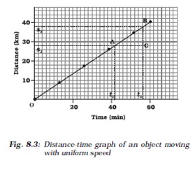
We know that when an object travels equal distances in equal intervals of time, it moves with uniform speed. This shows that the distance travelled by the object is directly proportional to time taken. Thus, for uniform speed, a graph of distance travelled against time is a straight line, as shown in Fig. 8.3. The portion OB of the graph shows that the distance is increasing at a uniform rate. Note that, you can also use the term uniform velocity in place of uniform speed if you take the magnitude of displacement equal to the distance travelled by the object along the y-axis. We can use the distance-time graph to determine the speed of an object. To do so, consider a small part AB of the distance-time graph shown in Fig 8.3. Draw a line parallel to the x-axis from point A and another line parallel to the y-axis from point B. These two lines meet each other at point C to form a triangle ABC. Now, on the graph, AC denotes the time interval (t₂ – t₁) while BC corresponds to the distance (s₂ – s₁). We can see from the graph that as the object moves from the point A to B, it covers a distance (s₂ – s₁) in time (t₂ – t₁). The speed, v of the object, therefore can be represented as

v = (s₂-s₁)/(t₂-t₁) (8.4)

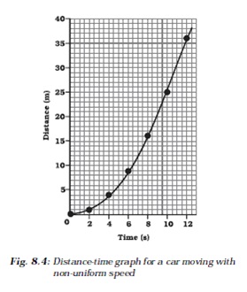
The distance-time graph for the motion of the car is shown in Fig. 8.4. Note that the shape of this graph is different from the earlier distance-time graph (Fig. 8.3) for uniform motion. The nature of this graph shows nonlinear variation of the distance travelled by the car with time. Thus, the graph shown in Fig 8.4 represents motion with non-uniform speed.

8.5 Equations of Motion by Graphical Method

When an object moves along a straight line with uniform acceleration, it is possible to relate its velocity, acceleration during motion and the distance covered by it in a certain time interval by a set of equations known as the equations of motion. There are three such equations. These are:

v = u + at (8.5)
s = ut + 1/2 at² (8.6)
2 a s = v² – u² (8.7)

where u is the initial velocity of the object which moves with uniform acceleration a for time t, v is the final velocity, and s is the distance travelled by the object in time t. Eq. (8.5) describes the velocity-time relation and Eq. (8.6) represents the position-time relation. Eq. (8.7), which represents the relation between the position and the velocity, can be obtained from Eqs. (8.5) and (8.6) by eliminating t. These three equations can be derived by graphical method.

8.5.1 EQUATION FOR VELOCITY-TIME RELATION

Consider the velocity-time graph of an object that moves under uniform acceleration as

We can also plot the distance-time graph for accelerated motion. Table 8.2 shows the distance travelled by a car in a time interval of two seconds.

shown in Fig. 8.8 (similar to Fig. 8.6, but now with u ≠ 0). From this graph, you can see that initial velocity of the object is u (at point A) and then it increases to v (at point B) in time t. The velocity changes at a uniform rate a. In Fig. 8.8, the perpendicular lines BC and BE are drawn from point B on the time and the velocity axes respectively, so that the initial velocity is represented by OA, the final velocity is represented by BC and the time interval t is represented by OC. BD = BC – CD, represents the change in velocity in time interval t.
Let us draw AD parallel to OC. From the graph, we observe that

BC = BD + DC = BD + OA

Substituting BC = v and OA = u,

we get v = BD + u

or BD = v -u (8.8)

From the velocity-time graph (Fig. 8.8), the acceleration of the object is given by

a = Change in velocity / timetaken

= BD / AD = BD / OC

Substituting OC = t, we get

a = BD t or BD = at (8.9)

Using Eqs. (8.8) and (8.9) we get

v = u + at

8.5.2 EQUATION FOR POSITION-TIME RELATION

Let us consider that the object has travelled a distance s in time t under uniform acceleration a. In Fig. 8.8, the distance travelled by the object is obtained by the area enclosed within OABC under the velocity-time graph AB.

Thus, the distance s travelled by the object is given by

s = area OABC (which is a trapezium)

= area of the rectangle OADC + area of the triangle ABD

= OA × OC + ½ (AD × BD) (8.10)

Substituting OA = u, OC = AD = t and BD = at, we get

s = u × t + ½(t×at)

or s = u t + 1/ 2 a t²

8.5.3 EQUATION FOR POSITION–VELOCITY RELATION

From the velocity-time graph shown in Fig. 8.8, the distance s travelled by the object in time t, moving under uniform acceleration a is given by the area enclosed within the trapezium OABC under the graph. That is,

s = area of the trapezium OABC

= {(OA + BC) × OC} / 2

Substituting OA = u, BC = v and OC = t,

we get

s = (u +v)t / 2 (8.11)

From the velocity-time relation (Eq. 8.6),

we get

t = (v – u ) / a (8.12)

Using Eqs. (8.11) and (8.12) we have

s = (v + u) × (v – u) / 2a

or 2 a s = v² – u²

8.6 Uniform Circular Motion

When the velocity of an object changes, we say that the object is accelerating. The change in the velocity could be due to change in its magnitude or the direction of the motion or both. Can you think of an example when an object does not change its magnitude of velocity but only its direction of motion?

Let us consider an example of the motion of a body along a closed path. Fig 8.9 (a) shows the path of an athlete along a rectangular track ABCD. Let us assume that the athlete runs at a uniform speed on the straight parts AB, BC, CD and DA of the track. In order to keep himself on track, he quickly changes his speed at the corners. How many times will the athlete have to change his direction of motion, while he completes one round? It is clear that to move in a rectangular track once, he has to change his direction of motion four times.

Now, suppose instead of a rectangular track, the athlete is running along a hexagonal shaped path ABCDEF, as shown in Fig. 8.9(b). In this situation, the athlete will have to change his direction six times while he completes one round. What if the track was not a hexagon but a regular octagon, with eight equal sides as shown by ABCDEFGH in Fig. 8.9(c)? It is observed that as the number of sides of the track increases the athelete has to take turns more and more often. What would happen to the shape of the track as we go on increasing the number of sides indefinitely? If you do this you will notice that the shape of the track approaches the shape of a circle and the length of each of the sides will decrease to a point. If the athlete moves with a velocity of constant magnitude along the circular path, the only change in his velocity is due to the change in the direction of motion. The motion of the athlete moving along a circular path is, therefore, an example of an accelerated motion.

We know that the circumference of a circle of radius r is given by 2πr . If the athlete takes t seconds to go once around the circular path of radius r, the velocity v is given by

v = (2πr)/t (8.13)

When an object moves in a circular path with uniform speed, its motion is called uniform circular motion.

Activity _____________8.11

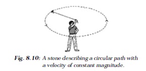
• Take a piece of thread and tie a small piece of stone at one of its ends. Move the stone to describe a circular path with constant speed by holding the thread at the other end, as shown in Fig. 8.10.

• Now, let the stone go by releasing the thread.
• Can you tell the direction in which the stone moves after it is released?
• By repeating the activity for a few times and releasing the stone at different positions of the circular path, check whether the direction in which the stone moves remains the same or not.

If you carefully note, on being released the stone moves along a straight line tangential to the circular path. This is because once the stone is released, it continues to move along the direction it has been moving at that instant. This shows that the direction of motion changed at every point when the stone was moving along the circular path.
When an athlete throws a hammer or a discus in a sports meet, he/she holds the hammer or the discus in his/her hand and gives it a circular motion by rotating his/her own body. Once released in the desired direction, the hammer or discus moves in the direction in which it was moving at the time it was released, just like the piece of stone in the activity described above. There are many more familiar examples of objects moving under uniform circular motion, such as the motion of the moon and the earth, a satellite in a circular orbit around the earth, a cyclist on a circular track at constant speed and so on.